Okabe-Ito Palette: Why It's the Gold Standard for Scientific Figures

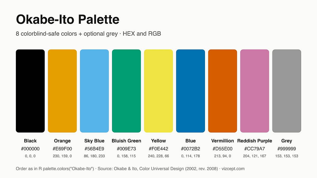
The Okabe-Ito palette is a set of eight Okabe-Ito colors (plus an optional neutral grey) designed by Masataka Okabe and Kei Ito to remain distinguishable to viewers with all three common types of color vision deficiency. Introduced through the Color Universal Design project in 2002 and popularized by Bang Wong in Nature Methods in 2011 (hence its nickname, the Wong palette), it is the most widely used colorblind-safe palette for categorical scientific figures — built into base R 4.0+ through palette.colors() and available as a ready-made scale in ggplot2 add-ons.

This guide gives you the copy-ready HEX and RGB codes plus R, Python, CSS and MATLAB snippets, then goes one layer deeper: where the Okabe-Ito palette actually came from, why those exact eight colors were chosen, when to use it versus the alternatives that have appeared since, and the common mistakes that quietly defeat its colorblind safety.

Building a colorblind-safe figure right now? Try the Scientific Color Palette Generator → — pick Okabe-Ito or any CVD-safe palette and copy hex codes in one click.

Who Made the Okabe-Ito (Wong) Palette, and Why?

The palette comes from the Color Universal Design (CUD) project led by Masataka Okabe at Jikei Medical School and Kei Ito at the University of Tokyo. Both authors are themselves strong protanopes, as the CUD page's own byline notes, and their motivation was concrete: medical figures — genetic linkage maps, fluorescence channels, microscopy overlays — routinely looked indistinguishable to colorblind viewers. About 8% of men and 0.5% of women of Northern European descent have some form of color vision deficiency (CVD), roughly 300 million people worldwide.

Rather than guess at color choices, Okabe and Ito ran candidate colors through CVD simulators and verified distinctness across the three main forms of color vision deficiency:

• Protanopia — missing the L (red) cone; the most common type
• Deuteranopia — missing the M (green) cone
• Tritanopia — missing the S (blue) cone; rare but still meaningful

Milder forms — protanomaly, deuteranomaly and tritanomaly — shift the same cones rather than removing them, so a palette that survives the full dichromat cases also holds up for these more common anomalous trichromats.

The eight colors that survived all three tests became the published palette (the CUD page is dated 2002 and was revised in 2008). Nine years after the original page, designer Bang Wong republished the same set in his Nature Methods "Points of View" column (Wong, 2011), giving it a global audience. That single citation is why the palette is sometimes called the "Wong palette" — but the original work is Okabe and Ito's.

The Eight Okabe-Ito Colors: HEX, RGB and Design Rationale

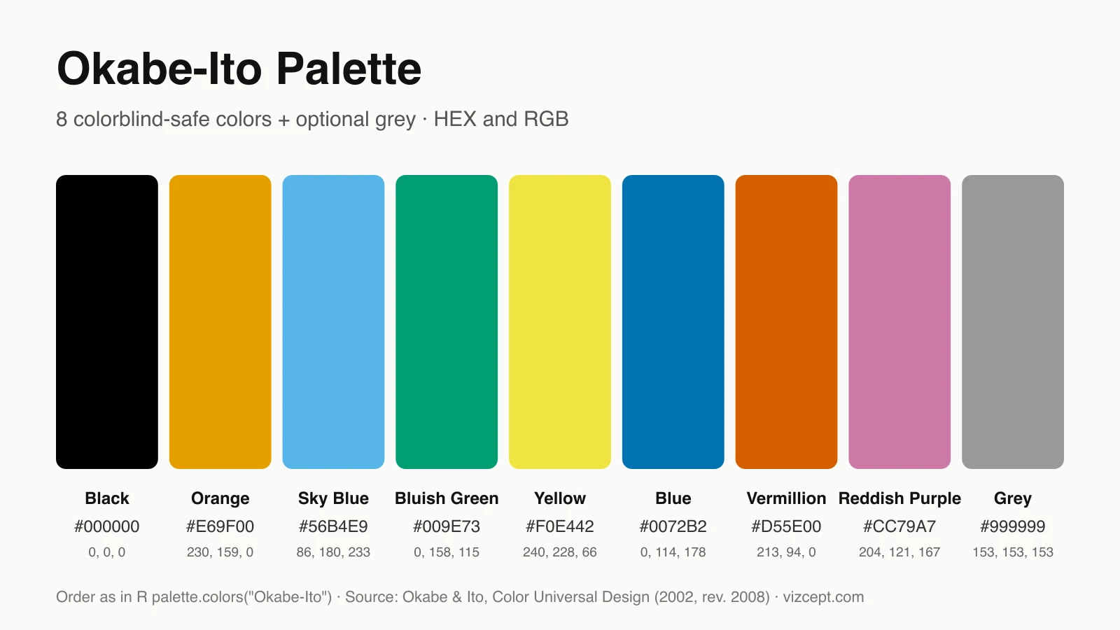
The Okabe-Ito palette is small on purpose. Going past eight categories makes any palette unreliable for CVD viewers, so the team stopped at eight:

#	Color	Hex	RGB	Why it's in the set
1	Orange	#E69F00	rgb(230, 159, 0)	High-luminance warm color, distinguishable from green under all CVD types
2	Sky Blue	#56B4E9	rgb(86, 180, 233)	Light blue, separated from blue by lightness and saturation rather than hue
3	Bluish Green	#009E73	rgb(0, 158, 115)	Replacement for "pure green" that collides with red under protanopia
4	Yellow	#F0E442	rgb(240, 228, 66)	The most luminant value in the set — survives grayscale
5	Blue	#0072B2	rgb(0, 114, 178)	Dark, saturated partner to sky blue; the darkest chromatic color in the set
6	Vermillion	#D55E00	rgb(213, 94, 0)	A "red" that retains its warmth under protanopia
7	Reddish Purple	#CC79A7	rgb(204, 121, 167)	Magenta variant that doesn't collapse into gray under deuteranopia
8	Black	#000000	rgb(0, 0, 0)	Reference / outline color

There's a quiet ninth slot too: a neutral grey (#999999) for background or "other" series. R's base implementation includes it as the ninth color, and many ports drop it.

Copy all eight Okabe-Ito hex codes in the recommended order:

#E69F00, #56B4E9, #009E73, #F0E442, #0072B2, #D55E00, #CC79A7, #000000

Ready-to-paste code for R, Python, CSS, MATLAB and GraphPad Prism is in How Do You Use the Okabe-Ito Palette in R, Python, CSS and MATLAB? below.

How the Okabe-Ito Palette Solves the Color Vision Problem

About 1 in 12 men has some form of CVD. The classic failure mode in scientific figures is the red-green collision: under protanopia and deuteranopia, the canonical "red line, green line" comparison looks nearly identical. The figure also fails in monochrome printouts — still common in print journals and lab notebooks.

The Okabe-Ito palette solves this three ways:

1. No pure red, no pure green. Vermillion (#D55E00) and bluish green (#009E73) sit far enough off the red-green axis to remain distinguishable under all three CVD types.
2. Wide luminance variation. Lightness runs from blue at L* ≈ 46 to yellow at L* ≈ 89, so many pairs still separate when desaturated. Not all of them do — see the lightness table below.
3. Maximum hue rotation. The set is roughly evenly spaced around the hue wheel, so even when two adjacent series share luminance, their hue contrast carries the distinction.

You can verify this with a CVD simulator such as Coblis, Color Oracle, Sim Daltonism or the dichromat R package. The figure below runs the Okabe-Ito colors and ggplot2's default hues through the same simulation:

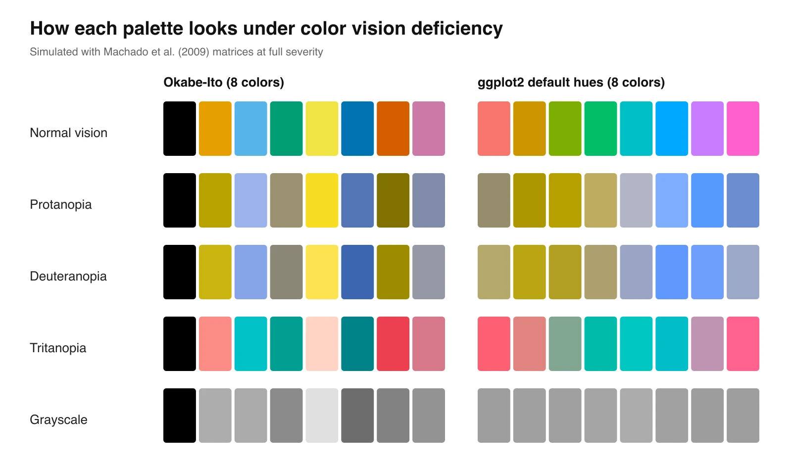
The default hues collapse into a band of olive and blue under protanopia and deuteranopia, and into nearly identical greys in grayscale. The Okabe-Ito colors keep more separation, but they are not perfect — which is why the lightness numbers matter.

How Light Is Each Okabe-Ito Color?

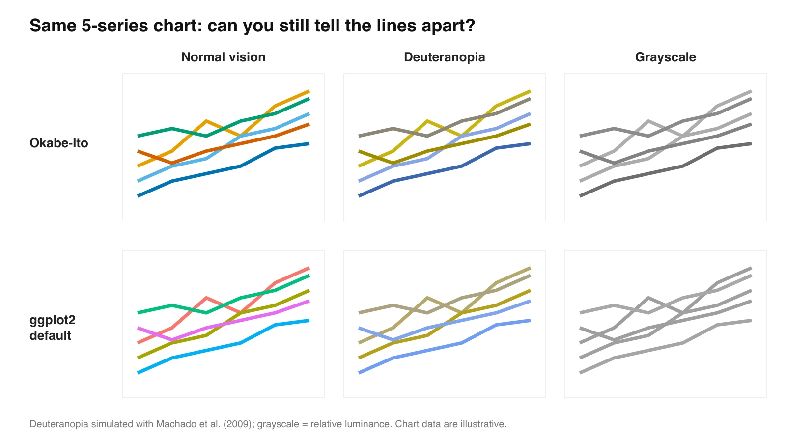
Two pairs are almost identical in lightness: orange and sky blue (L* 70.6 vs 69.8) and bluish green and vermillion (57.7 vs 54.2). In a grayscale print those pairs rely on hue alone, so give them different marker shapes or line styles. For text and thin lines, only blue (and black) clears WCAG's 4.5:1 contrast on a white background.

Color	HEX	L*	Contrast on white	Contrast on black
Blue	#0072B2	46.0	5.19:1	4.05:1
Vermillion	#D55E00	54.2	3.87:1	5.43:1
Bluish Green	#009E73	57.7	3.42:1	6.14:1
Reddish Purple	#CC79A7	61.0	3.06:1	6.86:1
Grey	#999999	63.2	2.85:1	7.37:1
Sky Blue	#56B4E9	69.8	2.31:1	9.10:1
Orange	#E69F00	70.6	2.25:1	9.32:1
Yellow	#F0E442	89.1	1.32:1	15.88:1

L* is CIELAB lightness (D65); contrast ratios follow the WCAG 2 relative-luminance formula. Yellow at 1.32:1 on white is the one to watch: keep it for filled areas and thick bars, never for thin lines or labels.

When to Use the Okabe-Ito Palette (and When Not To)

The Okabe-Ito palette is built for categorical data — discrete groups with no inherent order. It is not a sequential or diverging palette. The decision tree:

• Categorical, ≤ 8 groups, accessibility matters → Okabe-Ito ✓
• Categorical, ≥ 9 groups → Paul Tol's "muted" (9 colors), or facet your data into smaller subplots
• Sequential / ordered data (a continuous variable) → Viridis, Cividis, Magma
• Diverging (positive vs negative around zero) → ColorBrewer RdBu, PiYG, or Tol's "sunset"
• Heatmap / spatial → Viridis, Inferno
• Brand or marketing materials → not Okabe-Ito; the colors are tuned for distinctness, not emotion

A common misuse is treating the Okabe-Ito palette as a gradient by picking 3–5 of its colors as a low/medium/high scale. They aren't designed for that — they're maximally different, not stepwise. Reach for Viridis or Cividis when you need an ordered scale that also happens to be colorblind-safe.

Which Okabe-Ito Colors Should You Use for 2, 3 or 4 Groups?

You rarely need all eight. A dependable picking order for small groups:

• 2 groups → orange #E69F00 + blue #0072B2 (far apart in both hue and lightness)
• 3 groups → add bluish green #009E73
• 4 groups → add vermillion #D55E00, and give it a different marker shape from bluish green, since the two are close in lightness

Save yellow for last and keep it off thin lines. A common real-world example is a volcano plot: vermillion for up-regulated, blue for down-regulated and grey #999999 for non-significant genes.

Okabe-Ito Palette vs Other Colorblind-Safe Palettes

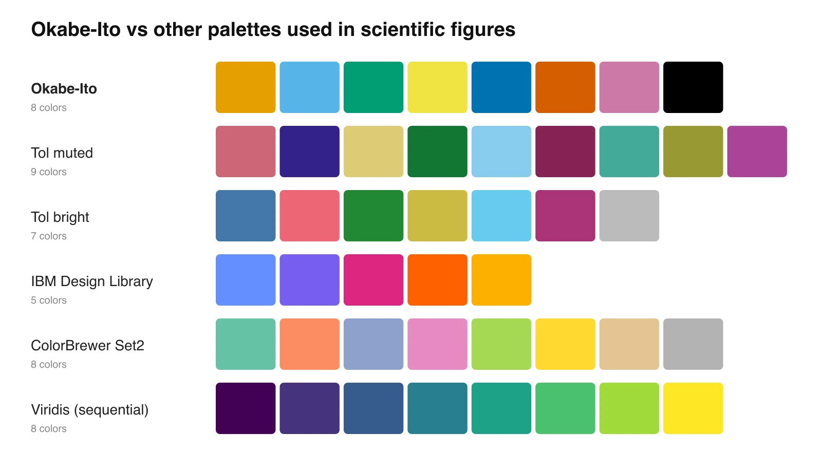
The CVD-safe palette space has grown a lot since the CUD page was revised in 2008. Here is how the Okabe-Ito palette stacks up against the modern alternatives most cited in scientific style guides:

Palette	Type	# Colors	Strength	Limitation
Okabe-Ito	Categorical	8	Most widely adopted; saturated; journal-ready	Hard cap at 8
Tol "muted"	Categorical	9	One extra color; explicit grey for "missing data"	Lower saturation; harder to project
Tol "bright"	Categorical	7	Higher contrast than muted	Fewer slots
IBM Design Library	Categorical	5	Web-tuned; designed for dashboards	Only 5 colors
Viridis	Sequential	Continuous	Perceptually uniform; CVD-safe across the gradient	Not for categorical data
ColorBrewer Set2	Categorical	8	Soft pastel feel	Not CVD-tested as rigorously

For categorical scientific figures with ≤ 8 groups, the Okabe-Ito palette remains the strongest default. For dashboards where the palette competes with brand colors, IBM's set integrates more easily. For more than 8 categories, Paul Tol's "muted" buys you one slot and a clean grey for missing data — at the cost of saturation.

A useful third source: the R Journal 2023 article "Coloring in R's Blind Spot" explains the color palettes added in R 4.0, including why Okabe-Ito was chosen as the default for palette.colors().

Where the Okabe-Ito Palette Is Built In Today

You no longer have to type the hex codes by hand. Major scientific stacks ship Okabe-Ito as a first-class option:

• R 4.0+ — palette.colors() returns Okabe-Ito by default (nine colors, black first, grey #999999 last)
• ggplot2 via easystats see — scale_color_okabeito()
• ggplot2 via ggokabeito — scale_color_okabe_ito()
• ggplot2 via ggthemes — scale_colour_colorblind(black = FALSE) drops black, which readers often mistake for a baseline
• Python — the cmap package ships it as okabeito; matplotlib and seaborn need the hex list set once (code below)
• Observable / D3 — not in d3-scale-chromatic; pass the hex array to d3.scaleOrdinal()
• CSS variables — easy to hand-roll (code below)

Note that ggplot2 itself has no Okabe-Ito scale; you either use one of the add-ons above or pass the codes to scale_color_manual(). Our own Scientific Color Palette Generator also has Okabe-Ito built in. If you only make a few figures a month, our BioRender alternative comparison sets BioRender's subscription against cheaper options and their publishing rights.

How Do You Use the Okabe-Ito Palette in R, Python, CSS and MATLAB?

All snippets use the recommended order without black, which suits most plots with a white background. Add "#000000" back if you need an eighth series.

R and ggplot2

okabe_ito <- c("#E69F00", "#56B4E9", "#009E73", "#F0E442",
               "#0072B2", "#D55E00", "#CC79A7")

# Base R 4.0+: the palette is built in
palette(palette.colors(palette = "Okabe-Ito"))

# ggplot2: scale colors manually
library(ggplot2)
ggplot(mpg, aes(displ, hwy, colour = drv)) +
  geom_point(size = 2.5) +
  scale_color_manual(values = okabe_ito)   # scale_fill_manual() for bars

Python: matplotlib and seaborn

import matplotlib.pyplot as plt
from cycler import cycler

okabe_ito = ["#E69F00", "#56B4E9", "#009E73", "#F0E442",
             "#0072B2", "#D55E00", "#CC79A7"]

# matplotlib has no built-in Okabe-Ito cycle, so set it once
plt.rcParams["axes.prop_cycle"] = cycler(color=okabe_ito)

# seaborn
import seaborn as sns
sns.set_palette(okabe_ito)

CSS custom properties

:root {
  --okabe-orange: #E69F00;
  --okabe-sky-blue: #56B4E9;
  --okabe-bluish-green: #009E73;
  --okabe-yellow: #F0E442;
  --okabe-blue: #0072B2;
  --okabe-vermillion: #D55E00;
  --okabe-reddish-purple: #CC79A7;
  --okabe-black: #000000;
}

MATLAB

okabe_ito = [230 159 0; 86 180 233; 0 158 115; 240 228 66;
             0 114 178; 213 94 0; 204 121 167] / 255;
set(groot, 'defaultAxesColorOrder', okabe_ito);

GraphPad Prism

Prism has no palette import, so enter the eight HEX codes once and save them as a custom color scheme: open Format Graph, set each data set's color by HEX, then save the result as a color scheme you can apply to future graphs.

Where Is the Official Okabe-Ito Source, and How Do You Cite It?

The official source is Okabe and Ito's Color Universal Design page, How to make figures and presentations that are friendly to colorblind people, hosted at jfly (dated 20 November 2002, revised 2008). The palette itself appears there as "Set of colors that is unambiguous both to colorblinds and non-colorblinds", alongside the authors' advice on redundant coding and replacing red with vermilion.

For academic work, cite the original page and, if you want the widely read journal reference, Wong's column:

• Okabe, M., & Ito, K. (2008). Color Universal Design (CUD): How to make figures and presentations that are friendly to colorblind people. https://jfly.uni-koeln.de/color/
• Wong, B. (2011). Points of view: Color blindness. Nature Methods, 8(6), 441. https://doi.org/10.1038/nmeth.1618

Five Common Mistakes When Using the Okabe-Ito Palette

The palette is robust, but it can still be misused:

1. Treating it as ordered. The colors are designed to be maximally different, not stepwise. Don't pick three as a low/medium/high scale — use Viridis.
2. Mixing in non-palette colors. Adding a "ninth" color from outside the set (like a brand red) reintroduces CVD problems and breaks the perceptual balance.
3. Reducing saturation for "softness." Lower saturation collapses the distinctness margin. If a figure feels too loud, reduce the number of categories instead.
4. Ignoring the recommended order. Okabe and Ito specified an order optimized for first-encounter contrast. ggplot2 and base R both respect it — overriding it loses some safety margin.
5. Skipping the grayscale check. Even with a CVD-safe palette, always preview the figure in grayscale — orange and sky blue, or bluish green and vermillion, can collide there. Pair each color with a marker shape or line style; the CUD page calls this redundant coding.

Frequently Asked Questions

What is the Okabe-Ito palette?

A set of eight colors (plus an optional grey) designed by Masataka Okabe and Kei Ito in 2002 to remain distinguishable across the three main forms of color vision deficiency. It became the de facto standard for categorical scientific figures after Bang Wong cited it in Nature Methods in 2011.

Is the Okabe-Ito palette colorblind friendly?

Yes. It was designed specifically for CVD safety and empirically tested across protanopia, deuteranopia, and tritanopia. It also survives grayscale printing because the eight colors span a wide luminance range.

What are the 8 colors of Okabe-Ito?

Orange (#E69F00), sky blue (#56B4E9), bluish green (#009E73), yellow (#F0E442), blue (#0072B2), vermillion (#D55E00), reddish purple (#CC79A7), and black (#000000). The set also includes a recommended neutral grey (#999999).

Is the Okabe-Ito palette the same as the Wong palette?

Yes — they are the same eight colors. "Wong palette" is a common nickname because Bang Wong reused Okabe and Ito's set in his 2011 Nature Methods article, which reached a much wider audience than the original CUD webpage.

Can I use the Okabe-Ito palette commercially?

Yes. Okabe and Ito published the palette as a public design recommendation with no usage restrictions. You don't need attribution, though citing the original CUD page or Wong (2011) is good practice in academic work.

What if I need more than 8 colors?

Either split your data into facets so each subplot shows ≤ 8 series, switch to Paul Tol's "muted" palette (9 colors), or — if your data is actually ordered — use a sequential palette like Viridis. Don't try to extend Okabe-Ito with extra colors; it breaks the CVD-safety guarantee.

Does the 60/30/10 rule apply to the Okabe-Ito palette?

No. The 60/30/10 (sometimes 60/30/10/10) rule is a brand and interior design guideline — pick one dominant color (60%), one secondary (30%), and one accent (10%). The Okabe-Ito palette is a categorical scheme where every series gets equal visual weight on purpose: the goal is maximum distinctness across data groups, not aesthetic balance. Use the 60/30/10 rule for slide templates or UI, not for scientific figures.

How do I use the Okabe-Ito palette in ggplot2?

ggplot2 has no built-in Okabe-Ito scale. Pass the hex codes to scale_color_manual(values = ...) or scale_fill_manual(values = ...), or install an add-on: ggokabeito (scale_color_okabe_ito()), easystats see (scale_color_okabeito()) or ggthemes (scale_colour_colorblind()).

Which color combinations should I avoid for colorblind readers?

Avoid red with green, and red with brown or black, since protanopes see dark red as nearly black. The CUD page also warns against pairing yellow-green with yellow or orange. Use vermillion instead of pure red, bluish green instead of pure green, and always add a second cue such as shape or line style.

Is there an extended Okabe-Ito palette with more colors?

No official one. The original set has eight colors; R's palette.colors() adds grey #999999 as a ninth. Beyond that, facet the data or switch to a larger palette such as Paul Tol's "muted".